Contagion

A Scientist's Take on the Princeton Facebook Paper

Spechler and Cannarella's paper predicting the death of Facebook has been taking a lot of flak. While I do think there are some issues applying their model to Facebook and MySpace, they're not the ones that most people are citing.

The most common complaint about the Princeton Facebook paper that I've seen is that Facebook is not a disease. Facebook may not be a disease, but that doesn't mean a model that describes how diseases spread isn't a good model for how Facebook spreads. Models based on the disease spread analogy have been used for decades in marketing. The famous "Bass Model" is just a relabeled disease model. Frank Bass's original paper has been cited thousands of times and was named one of the ten most influential papers in Management Science. While it's received its fair share of criticism, the entirety of The Tipping Point is based on the disease spread analogy. Gladwell even writes, "... ideas and behavior and messages and products sometimes behave just like outbreaks of infectious disease."

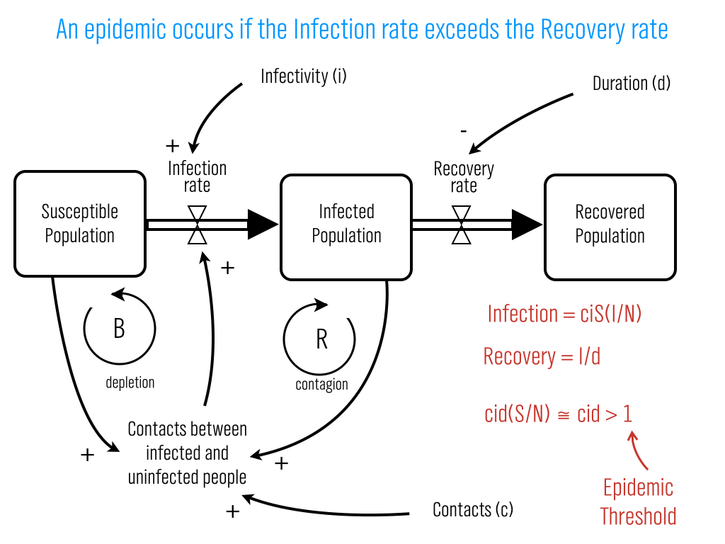
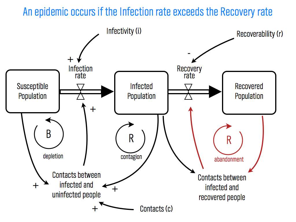
Interestingly, one of the major points of Spechler and Cannarela's paper is that online social networks do NOT spread just like a disease, that's why they had to modify the original SIR disease model in the first place. (See an explanation here.)

But, the critics have missed this point and are fixated on particulars of the disease analogy. For example, Lance Ulanoff at Mashable (who has one of the more evenhanded critiques) says, "How can you recover from a disease you never had?" He's referring to the fact that in Spechler and Cannarella's model, some people start off in the Recovered population before they've ever been infected. These are people who have never used Facebook and never will. It is a bit confusing that they're referred to as "recovered" in the paper, but if we just called them "people not using Facebook that never will in the future" that would solve the issue. Ulanoff has the same sort of quibble with the term recovery writing, "The impulse to leave a social network probably does spread like a virus. But I wouldn’t call it “recovery.” It's leaving that's the infection." Ok, fine, call it leaving, that doesn't change the model's predictions. Confusing terminology doesn't mean the model is wrong.

All of this brings up another interesting point, how could we test if the model is right? First off, this is a flawed question. To quote the statistician George E. P. Box, "... all models are wrong, but some are useful." Models, by definition, are simplified representations of the real world. In the process of simplification we leave things out that matter, but we try to make sure that we leave the most important stuff in, so that the model is still useful. Maps are a good analogy. Maps are simplified representations of geography. No map completely reproduces the land it represents, and different maps focus on different features. Topographic maps show elevation changes and road maps show highways. One kind is good for hiking the Appalachian trail, another is good for navigating from New York City to Boston. Models are the same — they leave out some details and focus on others so that we can have a useful understanding of the phenomenon in question. The SIR model, and Spechler and Cannarela's extension leave out all sorts of details of disease spread and the spread of social networks, but that doesn't mean they're not useful or they can't make accurate predictions.

myspace

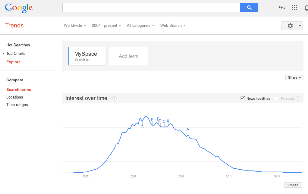
Spechler and Cannarela fit their model to data on MySpace users (more specifically, Google searches for MySpace), and the model fits pretty well. But this is a low bar to pass. It just means that by changing the model parameters, we can make the adoption curve in the model match the same shape as the adoption curve in the data. Since both go up and then down, and there are enough model parameters so that we can change the speed of the up and down fairly precisely, it's not surprising that there are parameter values for which the two curves match pretty well.

There are two better ways that the model could be tested. The first method is easier, but it only tests the predictive power of the model, not how well it actually matches reality. For this test, Spechler and Cannarela could fit the model to data from the first few years of MySpace data, say from 2004 to 2007, and see how well it predicts MySpace's future decline.

The second test is a higher bar to clear, but provides real validation of the model. The model has several parameters — most importantly there is an "infectivity" parameter (β in the paper) and a recovery parameter (γ). These parameters could be estimated directly by estimating how often people contact each other with messages about these social networks and how likely it is for any given message to result in someone either adopting or disadopting use of the network. For diseases, this is what epidemiologists do. They measure how infectious a disease is and how long ti takes for someone to recover, on average. Put these two parameters together with how often people come into contact (where the definition of "contact" depends on the disease — what counts as a contact for the flu is different from HIV, for example), and you can predict how quickly a disease is likely to spread or die out. (Kate Winslet explains it all in this clip from Contagion.) So, you could estimate these parameters for Facebook and MySpace at the individual level, and then plug those parameters into the model and see if the resulting curves match the real aggregate adoption curves.

Collecting data on the individual model parameters is tough. Even for diseases, which are much simpler than social contagions, it takes lab experiments and lots of observation to estimate these parameters. But even if we knew the parameters, chances are the model wouldn't fit very well. There are a lot of things left out of this model (most notably in my opinion, competition from rival networks.)

Spechler and Cannarella's model is wrong, but not for the reasons most critics are giving. Is it useful? I think so, but not for predicting when Facebook will disappear. Instead it might better capture the end of the latest fashion trend or Justin Bieber fever. 


Joshua Spechler and John Cannarella's Facebook is Dying Paper

This morning my email is blowing up with links to articles describing research by Joshua Spechler and John Cannarella, two Princeton PhD students, that predicts Facebook will lose 80% of its user base between 2015 and 2017. Are they right?

The paper is getting plenty of criticism, but as far as I can tell most of the critics haven't read or didn't understand the math in the paper. Let's take a closer look. Spechler and Cannarella's starting point is a basic model of disease spread called the SIR model. The SIR model (and its marketing variant the Bass model) have been applied to study the spread of innovations for decades. Without calling it by its name, I discussed applying the SIR model to the spread of memes online in the previous post on "What it Takes to Go Viral".

The SIR model is pretty simple. Imagine everyone in the world is in one of three states, Susceptible, Infected, or Recovered. Every time a Susceptible person bumps into an Infected person, there is a chance they become Infected too. Once a person is Infected, they stay Infected for awhile, but eventually they get better and become Recovered. The whole model is summed up by this "stock and flow" diagram.

SIR.001


Spechler and Cannarella update this model by making the recovery rate proportional to the number of recovered individuals. In other words, as more "recover" there is an increasing rate of recovery. In terms of Facebook, this would be interpreted as an increasing social pressure to leave Facebook as more other people leave Facebook. In our diagram, this amounts to adding another feedback loop — the "abandonment" feedback loop in red below:

SIRr.001.001


The effect of adding this loop is that recovery is slower in the beginning, because few people have recovered so there isn't much social pressure to recover, but then to accelerate recovery as the recovered population grows. For Facebook, it would mean once people start leaving, they'll leave in droves. When Specheler and Cannarella fit this model to the data, the best fit predicts that this mass exodus for Facebook will occur between 2015 and 2017.

To test their model they fit it to data on MySpace (they use Google Search data, which is a cool idea) and find that it fits pretty well. But, here's where we need to start being skeptical. First, just because the model fits the data well doesn't mean that the model captures what's really happening. It just means that you can manipulate the parameters of the model to produce a curve that goes up and down with a shape similar to the up and down curve that describes the users of MySpace over time. This isn't too surprising.

More problematic is that the model doesn't account for what is most likely the biggest single reason that people left MySpace — Facebook. In this model, the reason people leave MySpace is that everyone else is leaving MySpace — MySpace becomes uncool and there is a social pressure to not be on MySpace. But in reality, people probably didn't feel pressure to not be on MySpace, they left MySpace because they felt pressure to be on Facebook because that's where everyone else was.

I think this is an interesting model, but it's probably better suited to other phenomenon. When I was in junior high, it was cool to "tight roll" your jeans as demonstrated by these ladies.

tight-rolled-pants-3By the time I was in high school, no one would be caught dead tight rolling their jeans. This is the kind of dynamic that Spechler and Cannarella's model captures.

It's quite possible that Facebook will pass away, but probably only if something new comes along to displace it, not because people are embarrassed if someone finds out they still have an account.


Why Some Stories Go Viral (Maybe)

I read a(nother) article on Fast Company today about why some stories "go viral." (Mathematically speaking, why some things go viral and others don't boils down to a  simple equation.)

The article cites research by Jonah Berger and Katherine Milkman that finds articles with more emotional content, especially positive emotional content, are more likely to spread. A quick read of the article seems to promise an easy path to getting your own content on your blog, YouTube, or Twitter to take off. For example, the article cites Gawker editor Neetzan Zimmerman's success, pointing out his posts generate about 30 million views per month — the kind of statistics that get marketers salivating. The scientific research by Berger and Milkman is interesting and well done, but we have to be careful about how far we take the conclusions.

There are two interrelated issues. The first has to do with the "base rate." Part of Berger and Milkman's paper looks at what factors make articles on the New York Times online more likely to wind up on the "most emailed" list. They find, for example, that "a one standard deviation increase in the amount of anger an article evokes increases the odds that it will make the most e-mailed list by 34%."  In this case, the base rate is the percent of articles overall that make the most emailed list. When we hear that writing an especially angry article makes it 34% more likely to get on the most emailed list, it sounds like angry articles have a really good chance of being shared, but this isn't necessarily the case. What we know is that the probability of making the most emailed list given that the article is especially angry equal 1.34 times the base rate — but if the base rate is really low, 1.34 times it will be small too. Suppose for example that only 1 out of every 1000 articles makes the most emailed list, then what the result says is that 1.34 out of every thousand angry articles makes the most emailed list. 1.34 out of a thousand doesn't sound nearly as impressive as "34% more likely."

The second issue has to do with the overall predictability of making the most emailed list. The model that shows the 34% boost for angry content has an R-squared of .28. This model has more than 20 variables including things like article word count, topic, and where the article appeared on the webpage. But even knowing all of these variables, we still can't accurately predict if an article will make the most emailed list or not. All we know is that on average articles with some features are more likely to make the list than articles with other features. But for any particular article, we really can't do a very good job of predicting what's going to happen.

To get a better understanding of this idea, here's another example. In Ohio, 37% of registered voters are registered as Republicans and 36% are registered as Democrats. In Missouri, 39% are registered as Republicans and 37% are registered as Democrats. On average, registered voters in Missouri are more likely to be Republican than registered voters in Ohio, but just because someone is from Missouri doesn't mean we can confidently say they're a Republican. If we only looked at people from Ohio and Missouri, knowing which state a person is from wouldn't be a very good predictor of their party affiliation.

Obesity Epidemic?

Today on Slate there is a nice little GIF (that originally appeared on The Atlantic) that shows how obesity rates have changed over time by state. Slate seems to suggest that the geographic progression of obesity rates might indicate some sort of social contagion. But, ss many others (and here) before me have pointed out, we have to be very careful when trying to draw inferences about social contagion. If we take a look at a map of household income by state, we see that there is a lot of overlap between the poorest states and those with the highest obesity rates.

Household Income

There are lot's of potential causal connections here. For example, income might affect the types of stores and restaurants available, which in turn affects obesity rates. For a more careful look at some data on the social contagion of obesity, have a look at our paper that examines obesity rates, screen time, and social networks in adolescents.


As a side note, it's interesting to compare the map of the "obesity epidemic" to a map of something we know spreads through person to person contagion, like the swine flu (image from the New York Times).

H1N1

Unlike the obesity epidemic, swine flu jumps all over the place, which obviously has to do with air travel.

New paper on social contagion of obesity

Along with a team of researchers led by epidemiologist David Shoham from Loyola University, I recently published a paper in PLoS One examining the social contagion of obesity. As many of you know, this is a hotly debated topic of research that was kicked off by work of James Fowler and Nicholas Christakis published in the New England Journal of Medicine.  (See this post for my two cents on the debate.) The central criticism of this research surrounds the issue of separating friendship selection from influence, which in some sense was laid to rest by Cosma Shalizi and Andrew Thomas.

One alternative approach is to use a "generative model," which is exactly what my coauthors and I do. Specifically, we use the SIENA program developed by Tom Snijders and colleagues. Essentially, this model assumes that people make choices about their friendships and behavior just like economists and marketers assume people make choices about where to live or what car to buy.

In our paper, we apply the model to data from two high schools from the AddHeath study. We use the model to understand social influences on body size, physical activity, and "screen time" (time spent watching TV, playing video games, or on the computer). In short, here's what we find:

  • In both schools students are more likely to select friends that have a similar BMI (body mass index), that is there is homophily on BMI.
  • In both schools there is evidence that students are influenced by their friends' BMI.
  • There is no evidence for homophily on screen time in either school, and there is evidence that students are subject to influence from their friends'  on screen time in only one of the two schools.
  • In one of the two schools there was evidence for homophily on playing sports, but in both schools there was evidence that students influenced their friends when it comes to playing sports.

Visualizing Contagious Twitter Memes with NodeXL and Gephi

In the last post we explored how to use NodeXL to collect a Twitter user's network data. Now, I'll describe how to collect data on a trending topic.

To get started, follow steps 0 and 1 here to setup a Twitter account and download the NodeXL software. Then, to download the network data, click on Import and select From Twitter Search Network… In the first dialog box, enter the search term that you want to look for. Any account that recently posted a tweet containing this phrase will end up being a node in your network.  In the book, "Analyzing Social Media Networks with NodeXL," there is some good advice on choosing an appropriate trending topic to look at:

"First, the search phrase has to concern a recent event. Though Twitter has been around for several years, the volume of information being produced every second is so huge that the search interface has limits on how many tweets it will return for a given query, or how old tweets can be. Searching for "2008 Election" may in theory produce a valuable set of tweets about the election cycle, but in practice those tweets are too far back in time for the search interface to collect them efficiently. The second criterion is that the search phrase has to relate to a piece of news, promotion, event, and so on that is u contagious" (i.e., Twitter users who see the message will, at least in principle, want to pass it on to their followers). A search phrase like "Thanksgiving" is a trending topic on Twitter (shortly before and on Thanksgiving) but lacks a contagious property-there is no need to pass on the message because a large fraction of the population already knows about it, so tweets about Thanksgiving are independent events rather than the sign of a "Thanksgiving meme" spreading throughout the Twitter population."

One good way to do this is look through the recent tweets of a popular user for something that you think would be sufficiently interesting that other people would retweet the message. For example, in the network below, I gathered data on tweets containing the phrase "Who Googled You?" This Twitter meme originated with Pete Cashmore, of @mashable, and links to a Mashable article that describes a way to find out who has been searching for you on Google. The article generated a flurry of interest and many other people tweeted links to the article, generally repeating the original article title, "Who Googled You?" Since this meme spread from person to person, it was a good candidate for visualizing as a Twitter search network. Untitled

You can select what relationships you want to use to define the edges of your network by selecting any combination of the following choices:

Follows relationship — two accounts are connected if one account follows the other.
"Replies-to" relationship in tweet — two accounts are connected if one account replies to the other in its tweet.
"Mentions" relationship in tweet — two accounts are connected if one account mentions the other account in its tweet.

As discussed in the previous post, because of Twitter rate limits, it is advisable to limit your request to a fixed number of people. Unless you are especially patient, I recommend starting with just 300 people.

Once you download the data using NodeXL, I like to export it as a graphml file and then visualize it in Gephi. In this example, I did a few things to make the visualization more meaningful, which I describe below.

Before getting started with manipulating the network in Gephi, it is a good idea to go into the Data Laboratory and delete some of the columns that NodeXL created. You should delete anything having to do with the color or size of the nodes or edges, or centrality measures such as PageRank and eigenvector centrality. These columns are generally empty, but unless you delete them, Gephi won't overwrite them when you ask it to calculate these measures, so you won't be able to calculate and make use of them in your analysis. For some general tips on using Gephi, check out the FAQ here.

First, I filtered out all of the accounts except those that belong to the largest connected component of the network. This makes the network much more readable, and allows us to focus only on those nodes involved in a large cascade. After trying a few options, I choose the Force Atlas layout algorithm to arrange the nodes. For Twitter networks, I have found Force Atlas to generally give the best layout. Usually, I have to increase the repulsion strength from the default setting of 200 to 2000 or more. Then I resized the nodes according to their degree so we can get a sense for who the most important nodes in the network are. I also tried sizing the nodes by PageRank and eigenvector centrality for comparison. For the most part these different centrality measures didn't make much difference, although one account, @darrenmcd, appears significantly more important according to PageRank or Eigenvector centrality than degree centrality. The Twitter accounts @briansois and @armano standout as the most influential in the network. I colored the nodes according to which community they belong to as identified using Gephi's implementation of the Girvan-Newman modularity based clustering algorithm, and I colored the edges according to the type of relationship between the Twitter accounts. Blue edges are "followed" relationships, green edges are "mentions" and purple edges are "replies to." We can see that almost all of the links to @armano mention the relationship explicitly, and about half of those to @briansois do.

WhoGoogledYou

Of Monsters and Men — How an Icelandic Band Exploded using the Web

Bo Olafsson, a Kellogg student that took Social Dynamics and Networks with me this past fall quarter, put together a nice slideshow explaining how a little known Icelandic band, Of Monsters and Men, became a huge US success without ever visiting the country. Check it out:

Interestingly, Bo's slides have become a mini viral phenomenon themselves garnering press attention in both Iceland and the US:

What it takes to "Go Viral"

It seems like we hear a new story every week: a video, or a rumor, or a song, or a commercial has "gone viral," spreading across the web like wildfire, racing to the top of the most tweeted list, and grabbing headlines in real old fashioned news media. These memes can be disgusting (like the Domino's pizza video), controversial (like the recent Kony 2012 video), and entertaining ("Friday" ?). They can be disasters for companies (see Domino's above), or marketing campaigns that reach hundreds of thousand, or even millions, of viewers for relatively little investment (1300 foot drop, the Old Spice Guy). Given the potential impact of these "memes," there is a lot of interest in what exactly determines whether or not a video, or a message, or a rumor goes viral. Here's a simple model that explains why some things do and some things don't.

Let's consider the example of a YouTube video. Suppose that on average, every person that views the video tells of their friends about it per day (stands for contacts), and suppose that some fraction of the people that hear about the video actually watch it and start telling other people about it themselves (i stands for infectivity, and captures something like how interesting the video is.) Finally, suppose that on average, each person that is actively spreading word of the video does so for d days before they get bored and stop telling people about the video (d stands for duration).

To keep things simple, suppose that there are a total of N people in the population, and every one of these people is either actively spreading the video, or not actively spreading the video, but susceptible to becoming a video spreader. Let I denote the number of people currently spreading (i.e. infected) and S the number of people that are susceptible, but not currently spreading the video. So, I+S=N.

To see if the video goes viral or not, we just have to compare the rate at which people are becoming infected to the rate at which people are discontinuing sharing the video. It helps to think of a bath tub — the level of water in the bath tub represents the number of people spreading the video. The rate that water flows in through the faucet is the rate at which new people are becoming infected with the video spreading virus; the rate at which water drains out is the rate at which people are stopping spreading the video. If the rate at which water flows in is higher than the rate at which it drains out, the tub will keep filling up. On the other hand, if the drain is more open than the faucet, the bath tub will never fill up.

So, we have to figure out the rate at which new people are starting to spread the video and the rate at which people currently sharing the video are stopping. The second one is easier. If I people are currently sharing the video and each one of them shares it for d days on average, then each day we expect I/D people to stop spreading the video. For the first rate, we have I people actively sharing the video. On average, each one of them shares the video with c contacts per day, resulting in a total of cI contacts for the whole population. But, not all of these contacts results in a new person sharing the video. First, some of these people will already be sharing the video. The probability that a given person is not currently sharing the video is S/N, the fraction of "susceptible" people in the population. So, we expect cIS/N instances in which a person shares the video with someone that is currently spreading the video. Given such a contact, we said that a fraction i of these will result in a new person sharing the video. Putting it all together, the rate at which new people are becoming infected with the video sharing virus is ciIS/N.

Now we have to compare our two rates. The video will go viral if ciIS/N>I/d. Dividing both sides by I and multiplying both sides by d, this becomes, cidS/N>1. Finally, we can make life a little simpler by assuming that initially almost no one knows about the video, so the number of susceptible people S and the total population N are about the same. Then S/N is approximately 1, so the equation simplifies to just cid>1.

This simple equation tells us whether or not the video will go viral. It says if the average number of contacts, times the infectivity, times the duration is greater than one, the video will spread, otherwise it will die out. Right at cid=1 there is a tipping point; crossing this threshold causes a discontinuous jump in the future.

This model makes a lot of assumptions that don't really hold (big ones are that people have roughly the same # of contacts on average, and the people basically interact at random), but it gives us a basic understanding of the process. Even in more complicated models, where we make fewer simplifying assumptions, there is typically a similar tipping point, and increasing either contacts, infectivity, or duration increases the chance of crossing that threshold.

So, there you have it — everything you need to go viral: a network with enough contacts (c); a product, or message, that sounds interesting enough to be infectious (i), and with enough staying power so that people keep telling their friends about it for a long time (d).

Social Dynamics Videos

While I've been teaching Social Dynamics and Networks at Kellogg, I've amassed a collection of links to interesting videos on social dynamics. Here they are:

Duncan Watts TEDx talk on "The Myth of Common Sense"

Nicholas Christakis TED talk on "The hidden influence of social networks"; TED talk on "How social networks predict epidemics."

James Fowler talking about social influence on the Colbert Report.

Sinan Aral TEDx talk on "Social contagion"; at PopTech 2010 on "Social contagion"; at Nextwork on "Social contagion"; at the International Conference on Weblogs and Social Media on "Content and causality in social networks."

Scott E. Page on "Leveraging Diversity", and at TEDxUofM on "Putting Milk Crates on the Internet."

Eli Pariser TED talk on "Beware online 'filter bubbles'"

Freakonomics podcast on "The Folly of Prediction"

Damon Centola on "Network Contagion."

Jure Leskovec on "The Web as a Laboratory for Studying Humanity"

There are several good videos of talks from the Web Science Meets Network Science conference at Northwestern: Duncan Watts, Albert-Laszlo Barabasi, Jure Leskovec, and Sinan Aral.

The "Did You Know?" series of videos has some incredible information about, well, information. More info here.

Why Google Ripples will be a lot less cool than it sounds.

Google + now has a new feature, Ripples, that allows you to see a network visualization of the diffusion of a post (see the Gizmodo article here).  The pictures are cool, but the original post has to be public, and then it has to be shared by one Google+ user to other Google+ users.  But, the chance of interesting ripples happening very often are pretty slim; here's why.

Bakshy, Hofman, Mason, and Watts looked at exactly this kind of cascade on Twitter, which is a great platform for this kind of research for several reasons.  First, everything is effectively public, so there are none of the privacy issues of Facebook, and we don't have to limit ourselves to looking at just the messages that people choose to make public like we do on Google +.  Second, "retweeting" messages is an established part of Twitter culture, so we expect to find cascades. Finally, since tweets are limited to 140 characters, links are often shortened using services like bit.ly.  This means that if I create a link to a New York Times article and you create a link to the same page independently, those links will be different, so the researchers can tell the difference between a cascade that my post creates and one that yours creates.

Some of the cascades that Bakshy et al. found are shown in this figure.

They looked at 74 million chains like these initiated by more than 1.6 million Twitter users during two months in 2009.  A lot of interesting things came out of the study, but the most important one for Google Ripples is that 98 percent of the URLs were never reposted.  That's not good for Ripples.  The latest number puts the entire Google plus user population at only 43.6 million users, and since only a small fraction of these users' posts will be public posts, even if people share other people's posts on Google+ as frequently as the retweet links on Twitter (which is unlikely), we still can't expect to see many Ripples that look like anything but a lonely circle.